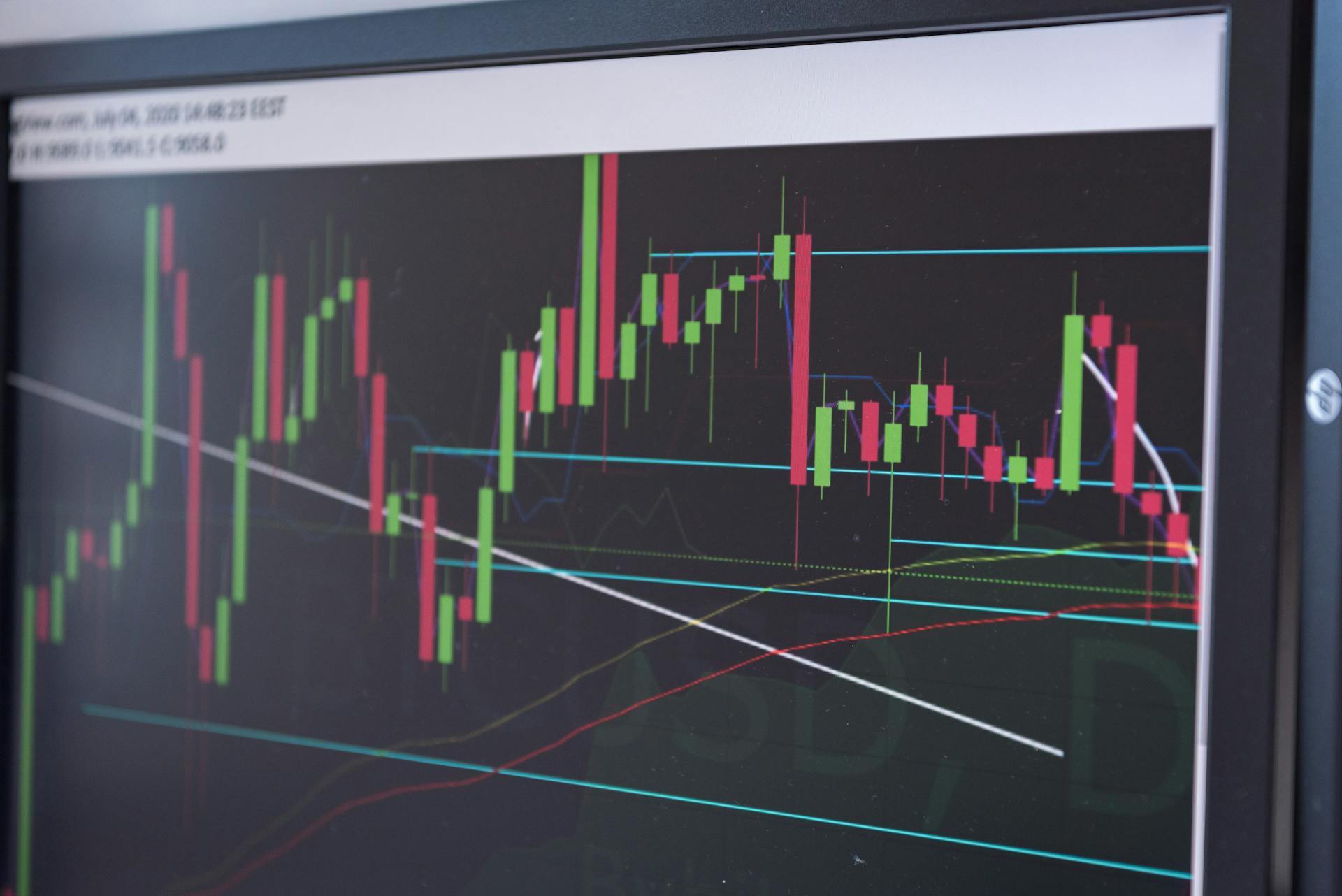
Stochastic Volatility Jump Fundamentals and Historical Perspective

Stochastic volatility jump models are used to capture the complex behavior of asset prices, particularly during periods of high volatility. These models are essential for risk management and portfolio optimization.

The concept of stochastic volatility was first introduced in the 1980s by John Cox, Jack Ingersoll, and Stephen Ross. This marked a significant shift in financial modeling, as it acknowledged that volatility is not constant, but rather a stochastic process that changes over time.

Stochastic volatility jump models are designed to account for both the volatility and jump risks in asset prices. This is crucial, as these risks can have a significant impact on portfolio performance.

Check this out: Stochastic Oscillator

Stochastic volatility jump models are commonly used to replicate stylized facts such as heavy tails and volatility clustering.

The advantage of these models is that they can capture sudden large movements in the price of an asset, which is a key feature of financial markets.

Merton's jump diffusion model, for example, extends the classic Black-Scholes model to include discontinuous asset returns, and the jumps are assumed to be independent from the diffusion.

Heston's stochastic volatility model, on the other hand, features a mean-reverting square-root process for the variance.

The combination of Merton's and Heston's models, as described by Bates (1996), allows for the replication of negative correlation between returns and volatility.

The stochastic differential equations (SDE) for the asset level and the variance under the risk-neutral measure are given by two correlated Brownian motions and a Poisson process for the jumps.

The jumps in the asset level SDE are assumed to be log-normally distributed with mean log-jump and standard deviation.

The choice of drift parameters that makes S_t e^(-rt) a martingale is given by the equation mu_t = r - lambda_t m, where m = E[J] - 1.

The variance process, on the other hand, is mean-reverting with mean reversion level, mean reversion strength, and constant volatility.

For another approach, see: Loss Given Default

Stochastic volatility jump models are used to capture the complex behavior of financial markets, particularly in times of high volatility.

These models assume that the underlying volatility is a stochastic process, meaning it can change over time. This is in contrast to traditional models that assume volatility remains constant.

The stochastic volatility jump model takes into account the possibility of sudden and unexpected jumps in the market, which can be caused by various factors such as economic announcements or natural disasters.

The model's ability to capture these jumps is particularly useful in times of high market stress, where traditional models may fail to accurately predict market behavior.

In fact, studies have shown that the stochastic volatility jump model can outperform traditional models in predicting stock prices during periods of high volatility.

The model's accuracy is due in part to its ability to account for the complex interactions between stock prices and volatility.

This is particularly evident in the model's ability to capture the "leverage effect", where an increase in volatility is associated with a decrease in stock prices.

Broaden your view: Stochastic Modelling (insurance)

Managing the risks associated with stochastic volatility jump is crucial for investors and financial institutions. This involves understanding the underlying causes of volatility and developing strategies to mitigate its impact.

The key to managing risk is to have a clear understanding of the underlying dynamics of stochastic volatility jump. This includes the role of jumps in asset prices and the impact of volatility on the behavior of financial markets.

A key factor in managing risk is the use of hedging strategies to offset potential losses. This can be achieved through the use of options, futures, and other derivatives.

Investors and financial institutions must also be prepared to adapt to changing market conditions. This requires continuous monitoring of market trends and the ability to adjust strategies as needed.

The use of advanced mathematical models, such as the Heston model, can also help to manage risk by providing a more accurate representation of stochastic volatility jump.

Check this out: Accounting and Auditing Organization for Islamic Financial Institutions

Stochastic volatility jump models can be challenging to implement in practice, but one effective strategy is to use a mixture of normal and lognormal distributions to capture the jump component. This approach can help to improve the accuracy of volatility forecasts.

A common method for estimating the parameters of a stochastic volatility model is the quasi-maximum likelihood estimator. This method is useful because it allows for the estimation of the model parameters without having to specify the distribution of the jumps.

The key to successful implementation of a stochastic volatility jump model is to carefully select the model parameters, such as the volatility of volatility and the jump size. A well-chosen set of parameters can make a significant difference in the accuracy of the model.

By using a combination of historical data and econometric techniques, investors can develop a robust investment strategy that takes into account the stochastic nature of volatility. This can help to reduce the risk of large losses due to unexpected market movements.

Additional reading: Stochastic Investment Model

Stochastic volatility jump models are designed to capture stylized facts of financial markets, such as heavy tails and volatility clustering.

The parameters of stochastic volatility models can be challenging to estimate, especially when incorporating jumps. This is because jumps require more estimating parameters compared to pure diffusion models.

The 3/2 stochastic volatility model with jump, for example, requires estimating parameters for the mean reversion level, mean reversion strength, and constant volatility of the variance process.

A key advantage of stochastic volatility jump models is their ability to replicate stylized facts, such as heavy tails and volatility clustering, which cannot be captured by traditional models like the Black-Scholes model.

Researchers have investigated various models, including the 3/2 model with jump, to better understand and estimate the parameters of stochastic volatility jump models.

The 3/2 model with jump effectively encompasses key market characteristics, but requires more estimating parameters compared to the pure diffusion model.

Check this out: Patricia Lopez / Bloomberg Opinion

Here are some key parameters involved in estimating the 3/2 model with jump:

These parameters are crucial in understanding and estimating the behavior of stochastic volatility jump models, and researchers continue to investigate and refine these models to better capture the complexities of financial markets.

In pure Lévy models, increments are stationary, but this lack of heteroscedasticity restricts their ability to fit the term-structure of implied volatilities.

The AD-DG jump-diffusion process, like any pure Lévy model, has stationary increments.

Its inability to fit the term-structure of implied volatilities is a significant limitation in financial modeling.

Incorporating a stochastic volatility component can help address this limitation, as it allows for more flexibility in fitting the term-structure of implied volatilities.

Related reading: Implied Enterprise Value

The historical perspective on volatility jumps is a rich and complex topic, reflecting the evolving understanding of market dynamics and the development of new analytical tools. From the early days of financial theory, the concept of volatility was central to the pricing of options and the management of risk.

The stock market crash of 1929 was a pivotal moment in the study of volatility jumps, prompting economists to reconsider the assumption of continuous market prices. This led to the development of models that could account for large, unpredictable changes.

Benoit Mandelbrot's work on Levy stable distributions and the Mandelbrotian random walk was a significant contribution to the understanding of volatility jumps. His work introduced the idea that real-world markets exhibit sudden, large movements not explained by normal distributions.

The 1970s saw the introduction of jump diffusion processes by Robert Merton, which incorporated both the continuous component of Black-Scholes and the discontinuous jumps. This marked a significant advancement in financial modeling.

The 1987 stock market crash, known as Black Monday, is a stark reminder of the market's susceptibility to jumps. Researchers analyzing high-frequency data have identified patterns of jumps, often clustering during periods of market stress.

Regulatory changes, such as the implementation of quantitative easing by central banks following the 2008 crisis, can also induce volatility jumps. The European sovereign debt crisis is another example of how macroeconomic policies can impact market volatility.

A different take: List of Oldest Banks in Continuous Operation

Keywords are an essential part of the research process. They help us find relevant information and narrow down our search results.

Following serials, authors, and keywords can make a big difference in our search results. It's like using a treasure map to find the hidden treasure!

Serials and authors can be used to find specific information on a topic. For example, following a particular author's work can give us insight into their research and ideas.

By using keywords, we can also find relevant information on a topic. Keywords can be words, phrases, or even hashtags that are related to our search query.

Following keywords can help us stay up-to-date on the latest research and trends in a particular field. It's like being part of a exclusive club that gets the latest scoop!

Suggestion: Which of the following Describes the Securities Underwriting Process

In finance, a fundamental trade-off often arises between generality and analytical tractability. This means that to achieve a more general asset price dynamics, we may have to sacrifice the type of solution it admits for the tail probability of the logarithmic return process.

The AD-DG jump-diffusion process is a pure Lévy model with stationary increments, which is a key characteristic. This implies that it can be calibrated to the market implied volatility smile of any single maturity.

However, its lack of heteroscedasticity restricts its ability to fit the term-structure of implied volatilities. This is a limitation that needs to be considered when working with the AD-DG model.

Incorporating a stochastic volatility component can help address this limitation, as I've done in my extension of the AD-DG dynamics. This extension involves deriving the characteristic function of logarithmic returns, which is a crucial step in pricing options.

Discover more: Dave Mccormick Ad