Arrow-Debreu Model of General Equilibrium Explained

The Arrow-Debreu model of general equilibrium is a groundbreaking concept in economics that revolutionized our understanding of how markets work. It was developed by economists Kenneth Arrow and Gerard Debreu in the 1950s.

This model is based on the idea that all markets are connected and that changes in one market can have a ripple effect on others. The model assumes that there are multiple markets, each with its own set of goods and services.

The model's key feature is that it shows how equilibrium can be achieved in a market with multiple goods, even if some of those goods are not traded directly. This is a crucial insight that has shaped the way economists think about market behavior.

The Arrow-Debreu model has had a lasting impact on the field of economics, influencing the development of new economic theories and models.

For your interest: Arrow Global

The Arrow–Debreu model is a complex economic model that attempts to describe how an economy functions. It consists of three main components: households, producers, and the market.

Households are the core of the model, and they are assumed to be utility maximizers, meaning they aim to consume the best possible bundle of commodities given their budget. They receive an endowment of commodities, which they can sell to the market, and they also receive dividends from the profits of the producers they own.

Producers, on the other hand, are assumed to be purely profit maximizers, and they transform bundles of commodities into other bundles to maximize their profits. The market is the mechanism that brings households and producers together, and it is assumed to be capable of "choosing" a market price vector that allows both households and producers to maximize their utility and profits.

The model assumes that households and producers have certain characteristics, such as the households having closed consumption sets, local nonsatiation, and convex preferences, and the producers having strictly convex production sets, no economies of scale, and the ability to close down for free.

Here are the assumptions made about households and producers in the Arrow–Debreu model:

Similarly, the model assumes that producers have strictly convex production sets, no economies of scale, and the ability to close down for free.

The model also assumes that the market is the mechanism that brings households and producers together, and it is assumed to be capable of "choosing" a market price vector that allows both households and producers to maximize their utility and profits.

The Arrow–Debreu model is a powerful tool for understanding how an economy functions, but it has its limitations, and it is not a realistic representation of how real-world economies work.

Related reading: How Do Quotas Help Domestic Producers

The Arrow–Debreu model is built around several key components that work together to create a comprehensive framework for understanding economic behavior. At its core, the model represents households and producers as separate entities.

A household's budget is determined by the sum of its income from selling endowments at the market price, plus profits from its ownership of producers. This is calculated using the formula Mi(p)=⟨p,ri⟩ +∑j∈Jαi,jΠj(p).

Each household has a Consumption Possibility Set (CPS), which represents the set of consumption plans it can afford. The CPS is determined by the household's budget and its preference relation over the consumption plans.

For another approach, see: Household Insurance Cover

Here are the key components of the Arrow–Debreu model:

These components work together to create a dynamic and complex economic system, where households and producers interact and make decisions based on their preferences and budget constraints.

Households are the building blocks of our economic model. Each household is indexed as i∈ ∈ I and begins with an endowment of commodities ri∈ ∈ R+N.

These commodities can be thought of as the household's initial resources, such as money or goods. Each household also begins with a tuple of ownerships of the producers α α i,j≥ ≥ 0, which represents their share of control over different producers.

The ownerships satisfy a specific condition: ∑ ∑ i∈ ∈ Iα α i,j=1∀ ∀ j∈ ∈ J. This means that for each producer, the sum of the ownerships of all households equals 1.

A household's budget is determined by the sum of its income from selling endowments at the market price, plus profits from its ownership of producers: Mi(p)=⟨ ⟨ p,ri⟩ ⟩ +∑ ∑ j∈ ∈ Jα α i,jΠ Π j(p).

Broaden your view: How Do You Sum a Column in Excel

Here's a breakdown of a household's budget:

Each household has a Consumption Possibility Set CPSi⊂ ⊂ R+N, which represents the set of all possible consumption plans they can choose from.

A consumption plan is a vector in CPSi, written as xi. The budget set is the set of consumption plans that a household can afford: Bi(p)=\{x^{i}\in CPS^{i}:\langle p,x^{i}\rangle \leq M^{i}(p)\}.

Readers also liked: Survey on Household Income and Wealth

In the economic model, producers and households are considered "price takers", meaning they accept market prices without influencing them.

This assumption helps simplify the model, but it's worth noting that behaviors like cartels and monopolies aren't accounted for.

Edgeworth's limit theorem suggests that households can't do better than price-take in an infinitely large economy.

In the Arrow–Debreu model, commodities can be broken down into smaller, more specific units to account for time, space, and uncertainty. This can be done by splitting one commodity into several, each contingent on a certain time, place, and state of the world.

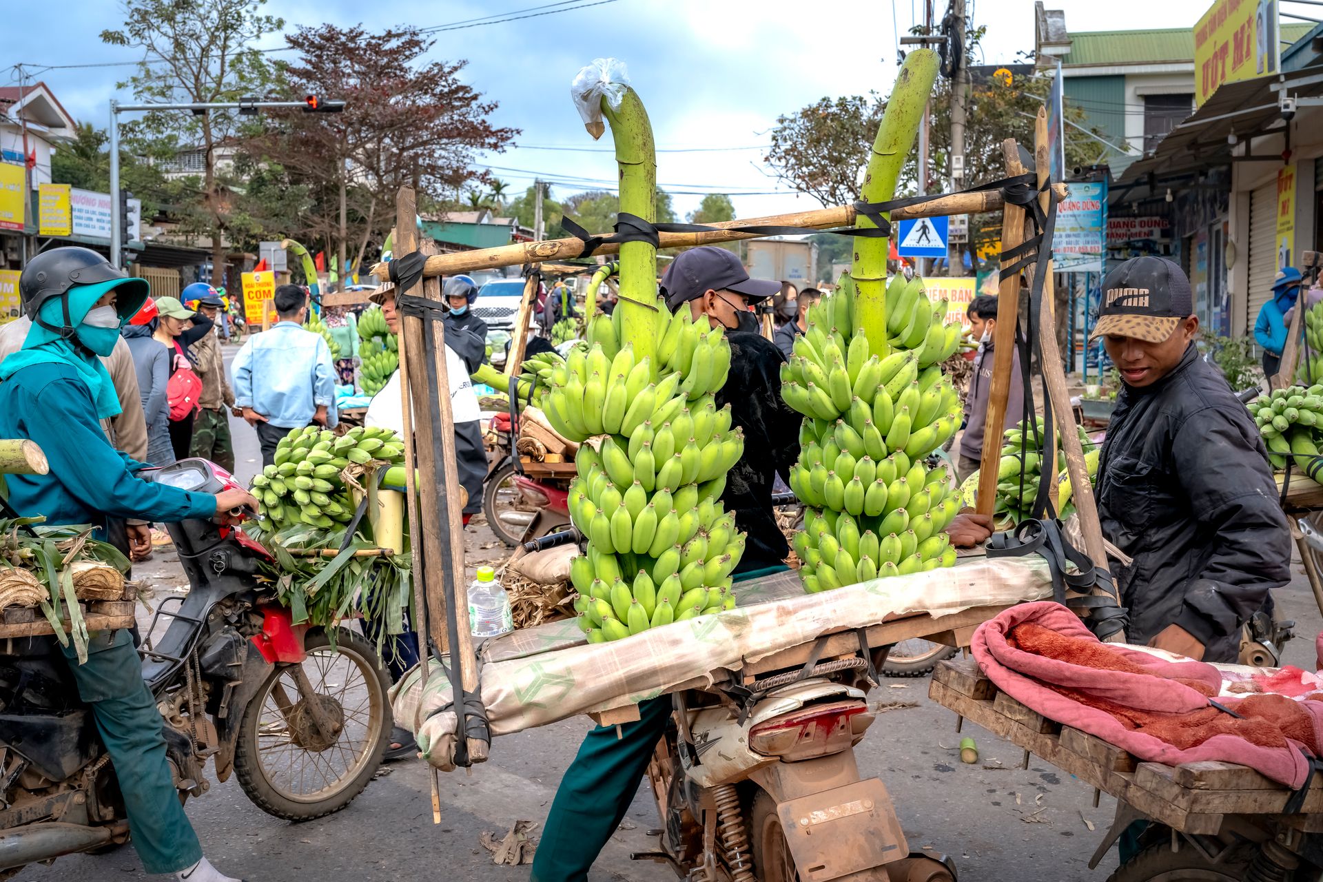
For example, "apples" can be divided into "apples in New York in September if oranges are available" and "apples in Chicago in June if oranges are not available". This allows for a more nuanced understanding of the market.

The Arrow–Debreu complete market is a market where there is a separate commodity for every future time, for every place of delivery, for every state of the world under consideration, for every base commodity. This is a key concept in the model.

A canonical Arrow–Debreu security is a security that pays one unit of numeraire if a particular state of the world is reached and zero otherwise. This is a fundamental component of the model.

Since the work of Breeden and Lizenberger in 1978, researchers have used options to extract Arrow–Debreu prices for various applications in financial economics. This has led to a deeper understanding of the model's implications.

In the Arrow–Debreu complete market, households and producers merely execute their planned productions, consumptions, and deliveries of commodities until the end of time. There is no need for storage of value or medium of exchange.

Related reading: 90-degree Arrow

An economy is a complex system that can be represented as a tuple (N,I,J,CPSi,⪰ ⪰ i,PPSj), which includes commodities, consumer preferences, consumption possibility sets, and producers' production possibility sets.

This tuple is the foundation of the Arrow-Debreu model, which represents the economy as a linear system. The model's representation allows us to use linear algebra techniques to analyze the existence and uniqueness of the competitive equilibrium.

The economy's state is a tuple of price, consumption plans, and production plans for each household and producer: ((pn)n∈ ∈ 1:N,(xi)i∈ ∈ I,(yj)j∈ ∈ J). This state is feasible if each xi∈ ∈ CPSi, each yj∈ ∈ PPSj, and ∑ ∑ i∈ ∈ Ixi⪯ ⪯ ∑ ∑ j∈ ∈ Jyj+r.

Here's a breakdown of the economy's components:

The economy is made up of many individual components, but to get a clear picture of the whole, we need to look at some key aggregates.

These aggregates are the sum of many individual parts, and they help us understand the overall state of the economy.

Aggregate consumption possibility set (CPS) is the sum of all individual consumption possibility sets. It's like adding up all the different ways people can spend their money.

The aggregate production possibility set (PPS) is the sum of all individual production possibility sets. This helps us see the total amount of goods and services that can be produced.

Here are some of the key aggregates in the economy:

The aggregate endowment is the total amount of resources available to the economy, and it's the sum of all individual endowments.

Aggregate demand and aggregate supply are also key aggregates, and they help us understand the overall level of economic activity.

The excess demand is the difference between aggregate demand and the sum of aggregate supply and the aggregate endowment.

Explore further: Cyclical Unemployment and Recession Often Arise from in Aggregate Demand.

An economy with an initial distribution is a crucial concept in understanding general equilibrium existence. An economy with initial distribution is an economy, along with an initial distribution tuple (ri,α α i,j)i∈ ∈ I,j∈ ∈ J{\displaystyle (r^{i},\alpha ^{i,j})_{i\in I,j\in J}} for the economy.

For another approach, see: Initial Public Offering of Facebook

The existence of general equilibrium is a fundamental question in economics. Ross M. Starr (1969) proved the existence of economic equilibria when some consumer preferences need not be convex. His proof used the Shapley–Folkman theorem.

A state of the economy is a tuple of price, consumption plans, and production plans for each household and producer: ((pn)n∈ ∈ 1:N,(xi)i∈ ∈ I,(yj)j∈ ∈ J){\displaystyle ((p_{n})_{n\in 1:N},(x^{i})_{i\in I},(y^{j})_{j\in J})}. A state is feasible iff each xi∈ ∈ CPSi{\displaystyle x^{i}\in CPS^{i}}, each yj∈ ∈ PPSj{\displaystyle y^{j}\in PPS^{j}}, and ∑ ∑ i∈ ∈ Ixi⪯ ⪯ ∑ ∑ j∈ ∈ Jyj+r{\displaystyle \sum _{i\in I}x^{i}\preceq \sum _{j\in J}y^{j}+r}.

The Arrow-Debreu Model represents the economy as a linear system, where the excess demand function is a linear function of the prices. This representation allows us to use linear algebra techniques to analyze the existence and uniqueness of the competitive equilibrium.

A state is an equilibrium state iff it is the state corresponding to an equilibrium price vector. An equilibrium price vector p{\displaystyle p} is an equilibrium price vector for the economy with initial distribution, iffZ(p)n{≤ ≤ 0 if pn=0=0 if pn>0{\displaystyle Z(p)_{n}{\begin{cases}\leq 0{\text{ if }}p_{n}=0\\=0{\text{ if }}p_{n}>0\end{cases}}}

You might like: Space Vector Corporation

Theorem—An equilibrium price vector exists for the restricted market, at which point the restricted market satisfies Walras's law. By definition of equilibrium, if p{\displaystyle p} is an equilibrium price vector for the restricted market, then at that point, the restricted market satisfies Walras's law.

Corollary—An equilibrium price vector exists for the unrestricted market, at which point the unrestricted market satisfies Walras's law.

Take a look at this: Vector Limited

The Arrow-Debreu model has some limitations that restrict its practical applications. One of these limitations is the assumption of convexity.

The assumption of convexity precluded many applications, which were discussed in the Journal of Political Economy from 1959 to 1961 by Francis M. Bator, M. J. Farrell, Tjalling Koopmans, and Thomas J. Rothenberg.

To overcome this limitation, economists have extended the model to infinite-dimensional economies, where the commodity space is infinite-dimensional. This requires the use of advanced mathematical techniques, such as functional analysis.

Intriguing read: Define Monetary Unit Assumption

An artificial restriction can be imposed on a market to study its behavior under certain conditions. This restriction is defined as a universal upper bound C, where every producer and household must use a production and consumption plan with a norm less than or equal to C.

The restriction is chosen to be "large enough" for the economy, meaning that the restriction is not in effect under equilibrium conditions. In detail, C is chosen to be large enough such that any consumption plan x with x ≥ 0 and ‖x‖ = C is "extravagant" and even if all producers coordinate, they would still fall short of meeting the demand.

For any list of production plans, if the sum of the production plans and the endowment r is non-negative, then each producer's individual production plan must lie strictly within the restriction.

At any price vector p, if the production plan of a restricted producer is interior to the artificial restriction, then the unrestricted producer would choose the same production plan.

If all production plans are equal to their restricted counterparts, then the restricted and unrestricted households have the same budget. If the consumption plan of a restricted household is interior to the artificial restriction, then the unrestricted household would choose the same consumption plan.

These two propositions imply that equilibria for the restricted market are equilibria for the unrestricted market.

Readers also liked: Jpmcb Large Cap Growth Fund

The Arrow-Debreu model of general equilibrium is based on a flawed assumption about the nature of equilibrium in a private property market economy. This model fails to accurately describe the real world and even as an idealized model, it makes a critical mistake.

The model assumes that ownership of production sets is a well-defined concept, but in reality, there is no such property right as "ownership of a production set" in a private property market economy. This ambiguity arises from the model's attempt to assign profits to individuals using the notion of "ownership of the production set."

The Arrow-Debreu model needs to assign residual claimancy to the corporation, but a simple argument shows that this is not necessary. Labor can hire capital, capital can hire labor, or a pure entrepreneur can hire both, making the concept of "ownership of a production set" irrelevant.

The model's failure to accurately describe the real world is an empirical commonplace, yet it is still widely accepted as representing the pure logic of the competitive market economy. However, this is not the case, and the model's limitations should be acknowledged.

Take a look at this: Concept of Money

The Uzawa equivalence theorem is a game-changer in economics, showing that the existence of general equilibrium is equivalent to Brouwer's fixed-point theorem. This means that we can use Brouwer's fixed-point theorem to prove the existence of equilibrium in general.

Walras's law is a fundamental concept in economics, stating that the value of a consumer's endowment is equal to the value of the goods they consume. This is represented mathematically as: ⟨ ⟨ p,r+∑ ∑ jyj⟩ ⟩ =c=⟨ ⟨ p,∑ ∑ ixi⟩ ⟩.

The two fundamental theorems of welfare economics hold without modification, thanks to the work of Uzawa. This is a significant result in economics, as it shows that certain theorems can be applied universally.

The excess demand function can be represented as a linear function of the prices, using the Arrow-Debreu Model. This representation allows us to use linear algebra techniques to analyze the existence and uniqueness of the competitive equilibrium.

Discover more: Nexi Fundamental

The Arrow-Debreu model makes some important assumptions about the shape of the supply and demand curves. These curves are actually convex, meaning they have a curved shape.

Convexity is a key concept in economics, and it's used to describe the relationship between prices and quantities. In the context of the Arrow-Debreu model, convexity means that the supply and demand curves are not strictly convex, but rather convex.

This modification changes the supply and demand functions from point-valued functions into set-valued functions, also known as correspondences. This is a more general case, and it's used to study markets where the supply and demand curves are not strictly convex.

Here's a comparison of the strictly convex case and the convex case:

In the convex case, the equilibrium exists by Kakutani's fixed-point theorem, which is a more general result than Brouwer's fixed-point theorem. This is an important result, as it shows that the Arrow-Debreu model can be used to study markets where the supply and demand curves are not strictly convex.

Convexity is a fundamental concept in economics, and it's essential to understand the difference between convexity and strict convexity. The assumptions of strict convexity can be relaxed to convexity, which changes supply and demand functions from point-valued functions into set-valued functions.

This modification allows for the application of Kakutani's fixed-point theorem, rather than Brouwer's fixed-point theorem. The generalization of the minimax theorem to the existence of Nash equilibria is also similar to this modification.

In the strictly convex case, PPSj is strictly convex, while in the convex case, it's just convex. The same goes for CPSi, which is strictly convex in the strictly convex case and convex in the convex case.

A key difference between the two cases is that the supply function S~ ~ j(p) is point-valued in the strictly convex case, but set-valued in the convex case. Additionally, the supply function is continuous in the strictly convex case, but has a closed graph (or is upper hemicontinuous) in the convex case.

The equilibrium exists by Brouwer's fixed-point theorem in the strictly convex case, but by Kakutani's fixed-point theorem in the convex case.

Recommended read: Negative Convexity Mbs

Market equilibrium assumes that every household performs utility maximization, subject to budget constraints.

The definition of market equilibrium involves maximizing utility while staying within a given budget, which can be represented as an optimization problem.

In this context, the dual problem is cost minimization subject to utility constraints, where the goal is to minimize the cost of achieving a certain level of utility.

The duality gap between the two problems is nonnegative, and may be positive, which means that some authors study the dual problem and the properties of its "quasi-equilibrium" (or "compensated equilibrium").

Every equilibrium is a quasi-equilibrium, but the converse is not necessarily true, highlighting a key distinction between the two concepts.

Additional reading: Dow Jones Utility Average

In economics, the concept of competitive equilibrium is a crucial one. It's a state where the market clears and all resources are allocated efficiently. This equilibrium exists when the supply and demand curves intersect.

According to the Arrow-Debreu Model, the competitive equilibrium exists and is unique under certain conditions. Specifically, if the excess demand function Z(p) is continuous, homogeneous of degree zero, and satisfies Walras' law, then a competitive equilibrium exists. This is a key result in the theory of general equilibrium.

See what others are reading: Cyber Insurance Demand

One of the most interesting aspects of the competitive equilibrium is that it can be interpreted in two ways: on the side of households and on the side of producers. On the side of households, it means that the aggregate household expenditure is equal to aggregate profit and aggregate income from selling endowments. In other words, every household spends its entire budget.

For an economy to have a competitive equilibrium, the excess demand function must satisfy certain conditions. It must be continuous, homogeneous of degree zero, and satisfy Walras' law. This is a strong requirement, but it's necessary for the existence of a competitive equilibrium.

There are several theorems that establish the existence and uniqueness of the competitive equilibrium. One of the most famous ones is the Arrow-Debreu theorem, which states that if the excess demand function is continuous and satisfies Walras' law, then there exists a competitive equilibrium. This theorem is a fundamental result in the theory of general equilibrium.

In some cases, an economy may have infinitely many equilibrium price vectors. However, "generically", an economy has only finitely many equilibrium price vectors. This means that for most economies, there are only a finite number of competitive equilibria.

The following table summarizes the conditions for the existence of a competitive equilibrium:

These conditions are necessary and sufficient for the existence of a competitive equilibrium. If an economy satisfies these conditions, then a competitive equilibrium exists and is unique.

Additional reading: Can You Change Medicare Supplement Plans with Pre Existing Conditions

In the Arrow-Debreu model, markets are assumed to be perfect, meaning that all agents have perfect knowledge of market conditions and can trade at any price.

Each agent's preferences are represented by a continuous utility function, which allows for infinite combinations of goods.

The model assumes that agents can trade all goods simultaneously, a concept known as a complete market.

This assumption is crucial for the model's results, as it allows for the existence of a competitive equilibrium.

The Arrow-Debreu model is often used to study the behavior of markets in equilibrium, where the supply and demand of goods are balanced.

A key feature of the model is the concept of a state-contingent commodity, which represents a good that can be traded in different states of the world.

This allows agents to hedge against uncertainty and take on risk in a way that's not possible in real-world markets.

The model's assumptions about market completeness and perfect knowledge are often criticized for being unrealistic, but they provide a useful framework for understanding the behavior of markets in theory.

Curious to learn more? Check out: Perfect Tender Rule

Computing general equilibria is a key aspect of the Arrow-Debreu model, and it's an area where Herbert Scarf made a significant breakthrough in 1967.

The Scarf algorithm is still widely used today to compute general equilibria, and it's a testament to the power of mathematical modeling in economics.

Scarf's work on this topic has been extensively reviewed and built upon by other researchers, including Kubler in 2012 and Scarf himself in 2018.

The stability of the competitive equilibrium is another crucial question in the Arrow-Debreu model, and it's one that can be addressed using linear algebra techniques.

The Jacobian matrix of the excess demand function is a key tool in this analysis, and it's defined as the partial derivative of the excess demand function with respect to prices.

The eigenvalues of the Jacobian matrix can be used to determine the stability of the equilibrium, and if all eigenvalues have negative real parts, the equilibrium is stable.

The Arrow-Debreu model represents the economy as a linear system, where the excess demand function is a linear function of prices.

This linear representation allows us to use linear algebra techniques to analyze the existence and uniqueness of the competitive equilibrium.

Readers also liked: Matrix Concepts Holdings

Linear algebra techniques are a crucial part of the Arrow-Debreu model. The excess demand function can be represented as a linear function of prices, allowing us to use linear algebra techniques to analyze the existence and uniqueness of the competitive equilibrium.

The Arrow-Debreu Model represents the economy as a linear system, where the excess demand function is a linear function of the prices. This representation is possible because the excess demand function can be represented as the sum of individual agent's excess demands.

Eigenvalues and eigenvectors can be used to analyze the stability of the competitive equilibrium. The eigenvalues of the Jacobian matrix of the excess demand function can be used to determine the stability of the equilibrium. If all eigenvalues have negative real parts, the equilibrium is stable.

Positive matrices play a crucial role in the Arrow-Debreu Model, representing the input-output structure of the economy. A positive matrix is a matrix with all positive entries, and positive matrices have several important properties, including the Perron-Frobenius theorem.

You might enjoy: Excess Reserves

In general, we write indices of agents as superscripts.

This is a crucial distinction to keep in mind, especially when working with complex equations.

Indices of agents are written as superscripts, which means they appear above the line of text.

This convention helps to avoid confusion between different types of indices.

For example, a vector coordinate index is written as a subscript.

Explore further: Does a Contract Have to Be Written

Linear algebra techniques can be used to represent the economy as a linear system, where the excess demand function is a linear function of the prices.

The Arrow-Debreu Model represents the economy as a linear system, allowing us to use linear algebra techniques to analyze the existence and uniqueness of the competitive equilibrium.

Linear algebra techniques can be used to analyze the stability of the competitive equilibrium by examining the eigenvalues of the Jacobian matrix of the excess demand function.

The Jacobian matrix is defined as the partial derivative of the excess demand function with respect to the prices, and its eigenvalues can be used to determine the stability of the equilibrium.

On a similar theme: Growth–share Matrix

Positive matrices play a crucial role in the Arrow-Debreu Model, representing the input-output structure of the economy.

A positive matrix is a matrix with all positive entries, and it has several important properties, including the Perron-Frobenius theorem, which states that a positive matrix has a unique largest eigenvalue, known as the Perron root.

The Perron-Frobenius theorem has significant implications for the analysis of the economy, as it provides a way to determine the largest eigenvalue of a positive matrix.

The eigenvalues of the Jacobian matrix can be used to determine the stability of the equilibrium, and if all eigenvalues have negative real parts, the equilibrium is stable.

The stability of the competitive equilibrium is an important question in the Arrow-Debreu Model, and linear algebra techniques provide a powerful tool for analyzing this question.

For another approach, see: The Most Important Thing Howard Marks

An economy is a complex system consisting of commodities, consumer preferences, consumption possibility sets, and producers' production possibility sets. This is represented as a tuple (N,I,J,CPSi,⪰ ⪰ i,PPSj){\displaystyle (N,I,J,CPS^{i},\succeq ^{i},PPS^{j})}, which specifies the various components of the economy.

Related reading: China Sets Worth Money

The state of an economy is a tuple of price, consumption plans, and production plans for each household and producer: ((pn)n∈ ∈ 1:N,(xi)i∈ ∈ I,(yj)j∈ ∈ J){\displaystyle ((p_{n})_{n\in 1:N},(x^{i})_{i\in I},(y^{j})_{j\in J})}. This state is feasible if each xi∈ ∈ CPSi{\displaystyle x^{i}\in CPS^{i}}, each yj∈ ∈ PPSj{\displaystyle y^{j}\in PPS^{j}}, and ∑ ∑ i∈ ∈ Ixi⪯ ⪯ ∑ ∑ j∈ ∈ Jyj+r{\displaystyle \sum _{i\in I}x^{i}\preceq \sum _{j\in J}y^{j}+r}.

A state is an equilibrium state iff it is the state corresponding to an equilibrium price vector. This means that if a commodity is not free, then supply exactly equals demand, and if a commodity is free, then supply is equal or greater than demand.

Consider reading: Uzbekistani Sum

An economy is a complex system that can be broken down into its core components. An economy is a tuple (N,I,J,CPSi,⪰ ⪰ i,PPSj){\displaystyle (N,I,J,CPS^{i},\succeq ^{i},PPS^{j})} that specifies the commodities, consumer preferences, consumption possibility sets, and producers' production possibility sets.

You might like: Two Sets of Books

In an economy, commodities are the goods and services that are produced and consumed. Consumer preferences refer to the individual tastes and preferences of households in the economy. Consumption possibility sets are the possible combinations of commodities that households can consume, given their income and prices.

Each household in the economy has a consumption possibility set (CPSi){\displaystyle CPS^{i}} that represents the possible combinations of commodities they can consume. Consumer preferences are represented by a relation ⪰ ⪰ i{\displaystyle \succeq ^{i}} that defines which consumption plans are preferred by the household.

Producers in the economy have production possibility sets (PPSj){\displaystyle PPS^{j}} that represent the possible combinations of commodities they can produce. A production plan is a vector in PPSj{\displaystyle PPS^{j}} that represents the specific combination of commodities produced by the producer.

A state of the economy is a tuple of price, consumption plans, and production plans for each household and producer. A state is feasible if each household's consumption plan is in their consumption possibility set, each producer's production plan is in their production possibility set, and the total demand for commodities is less than or equal to the total supply.

The feasible production possibilities set, given endowment r{\displaystyle r}, is PPSr:={y∈ ∈ PPS:y+r⪰ ⪰ 0}{\displaystyle PPS_{r}:=\{y\in PPS:y+r\succeq 0\}}. This set represents the possible combinations of commodities that can be produced, given the initial endowment of commodities.

Expand your knowledge: What Car Manufacturers Are Offering 0 Financing

Here are the key components of an economy:

Economic systems can be represented as linear systems, which allows us to use linear algebra techniques to analyze them.

This representation is based on the Arrow-Debreu Model, which represents the economy as a linear system where the excess demand function is a linear function of the prices.

The excess demand function can be represented as a sum of individual excess demand functions, where each function is a linear function of the prices.

The excess demand function can be written as Z(p) = ∑[z_i(p)], where z_i(p) is the excess demand of agent i at price p.

The number of terms in the sum represents the number of agents in the economy, which can be denoted as n.

The Arrow-Debreu Model allows us to use linear algebra techniques to analyze the existence and uniqueness of the competitive equilibrium.

Money can't be easily explained in a theoretical economy. In fact, it can't even be accounted for in an Arrow-Debreu economy.

The challenge of incorporating money into a theoretical economy is significant, as it's rarely a consideration for macroeconomists.

This lack of consideration is surprising, given that money is a fundamental aspect of our economic systems.

The most interesting and challenging aspect of money, from a theoretical standpoint, is that it doesn't fit into an Arrow-Debreu economy.

This should be a crucial consideration for macroeconomists, but it often gets overlooked in favor of more complex economic models.

Suggestion: Legal Definition of Consideration in Contract Law

The Arrow-Debreu model has some really cool applications in finance and macroeconomics.

In finance, the model is used to price assets and analyze the behavior of financial markets. This is achieved through the use of state prices, which allow us to value securities based on their potential payouts in different states of the world.

The model can also be used to study financial risk, which is a crucial aspect of financial economics. By understanding how state prices work, we can better manage risk and make more informed investment decisions.

One of the key benefits of the Arrow-Debreu model is its linearity, which makes it easy to value securities as the sum over all possible states of state price times payoff in that state. This is a game-changer for financial analysts and investors.

The model can be extended to infinite-dimensional economies, which requires the use of advanced mathematical techniques like functional analysis. This extension is useful for studying complex economic systems.

Here are some of the key applications of the Arrow-Debreu model in finance and macroeconomics:

The Arrow-Debreu model has been instrumental in helping us understand the behavior of financial markets and the economy as a whole. Its applications continue to grow and evolve, making it an essential tool for economists and financial analysts.

If you're interested in learning more about the Arrow-Debreu model, here are some related subjects to explore:

General Equilibrium is a fundamental concept that builds upon the Arrow-Debreu model, helping us understand how different economic agents interact and affect each other.

The History of Economic Thought and Methodology provides valuable context on how economic theories, including the Arrow-Debreu model, have evolved over time.

Mathematics plays a crucial role in the Arrow-Debreu model, making Mathematics in Business, Economics and Finance a relevant subject to explore.

Understanding Microeconomics is essential to grasping the Arrow-Debreu model, which focuses on individual economic units and their interactions.

Philosophy of Economics helps us think critically about the underlying assumptions and principles of economic theories, including the Arrow-Debreu model.

Quantitative Economics provides a framework for analyzing and solving economic problems, which is closely related to the mathematical underpinnings of the Arrow-Debreu model.

Here are some key related subjects to explore: